How to compare two columns in Excel for matches and differences

How to compare 2 columns in Excel row-by-row

When you do data analysis in Excel, one of the most frequent tasks is comparing data in each individual row. This task can be done by using the IF function, as demonstrated in the following examples.

Example 1. Compare two columns for matches or differences in the same row

To compare two columns in Excel row-by-row, write a usual IF formula that compares the first two cells. Enter the formula in some other column in the same row, and then copy it down to other cells by dragging the fill handle (a small square in the bottom-right corner of the selected cell). As you do this, the cursor changes to the plus sign:

Formula for matches

To find cells within the same row having the same content, A2 and B2 in this example, the formula is as follows:

=IF(A2=B2,"Match","")

Formula for differences

To find cells in the same row with different content, simply replace "=" with the non-equality sign:

=IF(A2<>B2,"No match","")

Matches and differences

And of course, nothing prevents you from finding both matches and differences with a single formula:

=IF(A2=B2,"Match","No match")

Or

=IF(A2<>B2,"No match","Match")

The result may look similar to this:

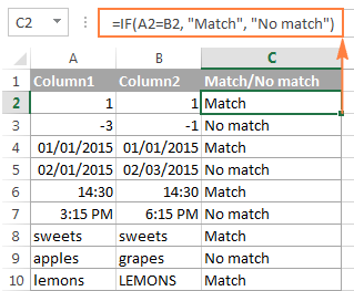
As you see, the formula handles numbers, dates, times and text strings equally well.

Example 2. Compare two lists for case-sensitive matches in the same row

As you have probably noticed, the formulas from the previous example ignore case when comparing text values, as in row 10 in the screenshot above. If you want to find case-sensitive matches between 2 columns in each row, then use the EXACT function:

=IF(EXACT(A2, B2), "Match", "")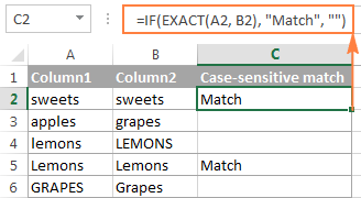

To find case-sensitive differences in the same row, enter the corresponding text ("Unique" in this example) in the 3^rd argument of the IF function, e.g.:

=IF(EXACT(A2, B2), "Match", "Unique")

Compare multiple columns for matches in the same row

In your Excel worksheets, multiple columns can be compared based on the following criteria:

• Find rows with the same values in all columns (Example 1)
• Find rows with the same values in any 2 columns (Example 2)

Example 1. Find matches in all cells within the same row

If your table has three or more columns and you want to find rows that have the same values in all cells, an IF formula with an AND statement will work a treat:

=IF(AND(A2=B2, A2=C2), "Full match", "")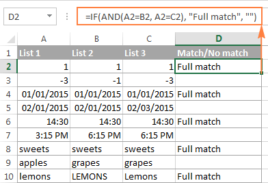

If your table has a lot of columns, a more elegant solution would be using the COUNTIF function:

=IF(COUNTIF($A2:$E2, $A2)=5, "Full match", "")

Where 5 is the number of columns you are comparing.

Example 2. Find matches in any two cells in the same row

If you are looking for a way to compare columns for any two or more cells with the same values within the same row, use an IF formula with an OR statement:

=IF(OR(A2=B2, B2=C2, A2=C2), "Match", "")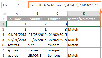

In case there are many columns to compare, your OR statement may grow too big in size. In this case, a better solution would be adding up several COUNTIF functions. The first COUNTIF counts how many columns have the same value as in the 1^st column, the second COUNTIF counts how many of the remaining columns are equal to the 2^nd column, and so on. If the count is 0, the formula returns "Unique", "Match" otherwise. For example:

=IF(COUNTIF(B2:D2,A2)+COUNTIF(C2:D2,B2)+(C2=D2)=0,"Unique","Match")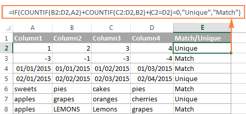

How to compare two columns in Excel for matches and differences

Suppose you have 2 lists of data in Excel, and you want to find all values (numbers, dates or text strings) which are in column A but not in column B.

For this, you can embed the COUNTIF($B:$B, $A2)=0 function in IF's logical test and check if it returns zero (no match is found) or any other number (at least 1 match is found).

For instance, the following IF/COUNTIF formula searches across the entire column B for the value in cell A2. If no match is found, the formula returns "No match in B", an empty string otherwise:

=IF(COUNTIF($B:$B, $A2)=0, "No match in B", "")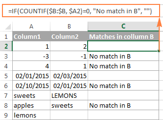

Tip. If your table has a fixed number of rows, you can specify a certain range (e.g. $B2:$B10) rather than the entire column ($B:$B) for the formula to work faster on large data sets.

The same result can be achieved by using an IF formula with the embedded ISERROR and MATCH functions:

=IF(ISERROR(MATCH($A2,$B$2:$B$10,0)),"No match in B","")

Or, by using the following array formula (remember to press Ctrl + Shift + Enter to enter it correctly):

=IF(SUM(--($B$2:$B$10=$A2))=0, " No match in B", "")

If you want a single formula to identify both matches (duplicates) and differences (unique values), put some text for matches in the empty double quotes ("") in any of the above formulas. For example:

=IF(COUNTIF($B:$B, $A2)=0, "No match in B", "Match in B")

How to compare two lists in Excel and pull matching data

Sometimes you may need not only match two columns in two different tables, but also pull matching entries from the second table. Microsoft Excel provides a special function for such purposes - the VLOOKUP function. As an alternative, you can use more powerful and versatile INDEX & MATCH formulas.

For example, the following formula compares the product names in columns D and A and if a match is found, a corresponding sales figure is pulled from column B. If no match is found, the #N/A error is returned.

=INDEX($B$2:$B$6,MATCH($D2,$A$2:$A$6,0))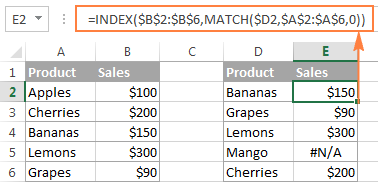

For the detailed explanation of the formula's syntax and more formula examples, please check out the following tutorial: INDEX & MATCH in Excel - a better alternative to VLOOKUP.

If you don't feel very comfortable with this formula, then you may want to try the Merge Tables wizard - a fast and intuitive solution that can compare and match 2 tables by any column(s).

Compare two lists and highlight matches and differences

When you compare columns in Excel, you may want to "visualize" the items that are present in one column but missing in the other. You can shade such cells in any color of your choosing by using the Excel Conditional Formatting feature and the following examples demonstrate the detailed steps.

Example 1. Highlight matches and differences in each row

To compare two columns and Excel and highlight cells in column A that have identical entries in column B in the same row, do the following:

• Select the cells you want to highlight (you can select cells within one column or in several columns if you want to highlight entire rows).
• Click Conditional formatting > New Rule… > Use a formula to determine which cells to format.
• Create a rule with a simple formula like =$B2=$A2 (assuming that row 2 is the first row with data, not including the column header). Please double check that you use a relative row reference (without the $ sign) like in the formula above.

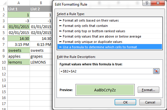
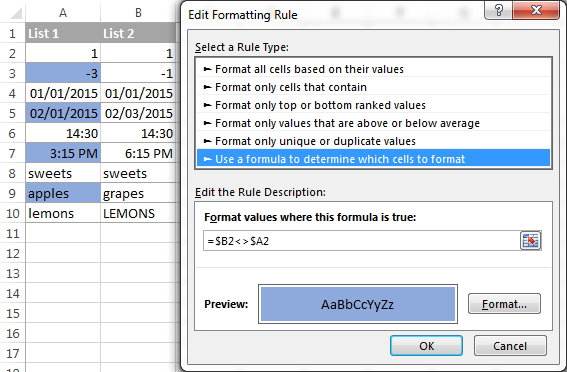
To highlight differences between column A and B, create a rule with the formula =$B2<>$A2

If you are new to Excel conditional formatting, please see How to create a formula-based conditional formatting rule for step-by-step instructions.

Example 2. Highlight unique entries in each list

Whenever you are comparing two lists in Excel, there are 3 item types that you can highlight:

• Items that are only in the 1^st list (unique)
• Items that are only in the 2^nd list (unique)
• Items that are in both lists (duplicates) - demonstrated in the next example.

This example demonstrates how to highlight items that are in one list only.

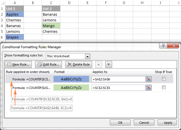
Supposing your List 1 is in column A (A2:A6) and List 2 in column C (C2:C5). You create the conditional formatting rules with the following formulas:

Highlight unique values in List 1 (column A): =COUNTIF($C$2:$C$5, $A2)=0

Highlight unique values in List 2 (column C): =COUNTIF($A$2:$A$6, $C2)=0

And get the following result:

Example 3. Highlight matches (duplicates) between 2 columns

If you closely followed the previous example, you won't have difficulties adjusting the COUNTIF formulas so that they find the matches rather than differences. All you have to do is to set the count greater than zero:

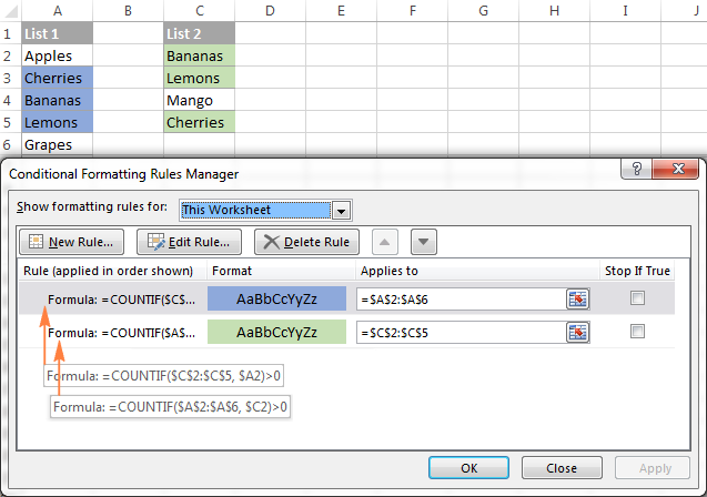
Highlight matches in List 1 (column A): =COUNTIF($C$2:$C$5, $A2)>0

Highlight matches in List 2 (column C): =COUNTIF($A$2:$A$6, $C2)>0

Example 4. Built-in rule to compare 2 lists and highlight duplicates or uniques

If you are one of those power users who mostly rely on functions and formulas, you may have missed this amazingly simple way to compare two columns in Excel :)

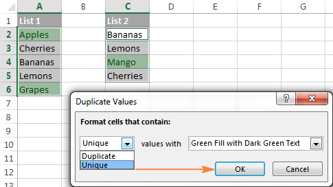
• Select two lists you want to compare. If they include different numbers of cells or are located in non-adjacent columns, select the first list, press and hold the Ctrl key, and then select the second list.
• On the Home tab, go to Conditional Formatting > Highlight Cells Rules > Duplicate Values.
• Select either Duplicate or Unique from the left-hand side drop-down list, and choose the desired format from the right-hand side drop-down. If you are not happy with any of the predefined formats, click Custom format… and set the Font or Fill color to your liking.
• Click OK and you are done!

Highlight row differences and matches in multiple columns

When comparing values in several columns row-by-row, the quickest way to highlight matches is creating a conditional formatting rule, and the fastest way to shade differences is embracing the Go To Special feature, as demonstrated in the following examples.

Example 1. Compare multiple columns and highlight row matches

To highlight rows that have identical values in all columns, create a conditional formatting rule based on one of the following formulas:

=AND($A2=$B2, $A2=$C2)

or

=COUNTIF($A2:$C2, $A2)=3

Where A2, B2 and C2 are the top-most cells and 3 is the number of columns to compare.

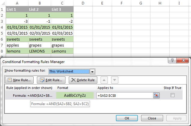
Of course, neither AND nor COUNTIF formula is limited to comparing only 3 columns, you can use similar formulas to highlight rows with the same values in 4, 5, 6 or more columns.

Example 2. Compare multiple columns and highlight row differences

To quickly highlight cells with different values in each individual row, you can use Excel's Go To Special feature.

1. Select the range of cells you want to compare. In this example, I've selected cells A2 to C8.
   
   By default, the top-most cell of the selected range is the active cell, and the cells from the other selected columns in the same row will be compared to that cell. As you can see in the screenshot above, the active cell is white while all other cells of the selected range are highlighted. In this example, the active cell is A2, so the comparison column is column A.
   To change the comparison column, use either the Tab key to navigate through selected cells from left to right, or the Enter key to move from top to bottom.
   Tip. To select non-adjacent columns, select the first column, press and hold Ctrl, and then select the other columns. The active cell will be in the last column (or in the last block of adjacent columns). To change the comparison column, use the Tab or Enter key as described above.
2. On the Home tab, go to Editing group, and click Find & Select > Go To Special… Then select Row differences and click the OK button.
   
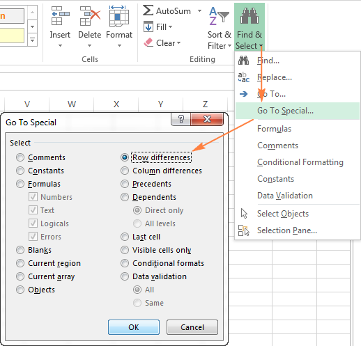
3. The cells whose values are different from the comparison cell in each row are highlighted.If you want to shade the highlighted cells in some color, simply click the Fill Color icon on the ribbon and select the color of your choosing.
   

How to compare two cells in Excel

In fact, comparing 2 cells is a particular case of comparing two columns in Excel row-by-rowexcept that you don't have to copy the formulas down to other cells in the column.

For example, to compare cells A1 and C1, you can use the following formulas:

For matches: =IF(A1=C1, "Match", "")

For differences: =IF(A1<>C1, "Difference", "")

To learn a few other ways to compare cells in Excel, please see How to compare strings in Excel.

For more powerful data analysis, you may need more sophisticated formulas and you can find a few good ideas in the following tutorials:

• Using IF function in Excel
• Nested IF with multiple conditions, IFERROR, IFNA and more

Formula-free way to compare two columns / lists in Excel

Now that you know Excel offerings for comparing and matching columns, let me demonstrate you an alternative solution that can compare 2 lists with a different number of columns for matches (duplicates) and differences (unique values).

Ablebits Duplicate Remover for Excel can search for identical and unique entries within one table as well as compare two tables residing on the same sheet or in 2 different worksheets / workbooks.

For the purpose of this article, we will be focusing on the second feature, which is called Compare Two Tables and is specially designed for comparing two lists by any column(s) that you specify. The comparison of two data sets by several columns is a real challenge both for Excel formulas and conditional formatting, but this tool handles it with ease.

Compare 2 lists by several columns in 6 quick steps

Supposing you have 2 tables of data and you want to find duplicate rows based on 3 columns - Date, Item and Sales:

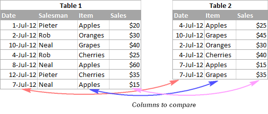
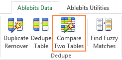
Step 1. Assuming that you have the Duplicate Remover for Excel installed, select any cell within the 1^st table, and click the Compare Two Tables button on the ribbon to start the wizard. This button resides on the Ablebits Data tab, in the Dedupe group.

Step 2. The wizard picks the entire table and suggests to create a backup copy of the original table, just in case. So, simply make sure your 1^st table is selected correctly and click Next.

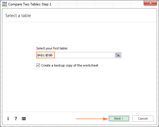
Step 3. Select the 2^nd table by using the standard Select range icon . If both tables reside in the same workbook and have similar column names, there's a great chance that the second list will be fetched automatically as well.

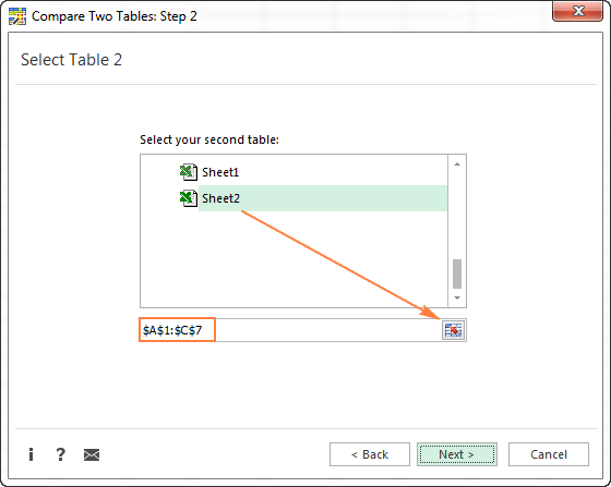
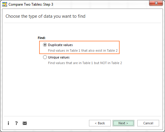
Step 4. Select whether to search for matches or differences:

• Duplicate values - look for matches, i.e. items that exist in both tables.
• Unique values - look for differences, i.e. items that are in Table 1 but not in Table 2.

In this example, we select Duplicate values and click Next.

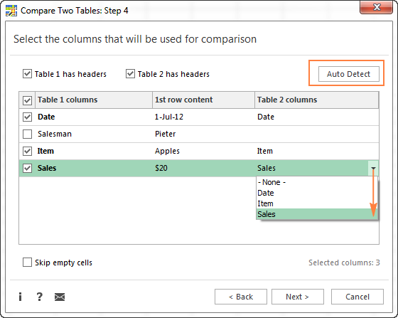
Step 5. This is the key step where you select the column pairs you want to compare in 2 tables. In this example, we are comparing 3 columns - Date, Item and Sales.

For the wizard to find the matching columns automatically, click the Auto Detect button in the upper-right corner. If the columns have different names in both tables, you might need to select the right column manually by clicking the little black arrow next to the Table 2 column on the right-hand side:

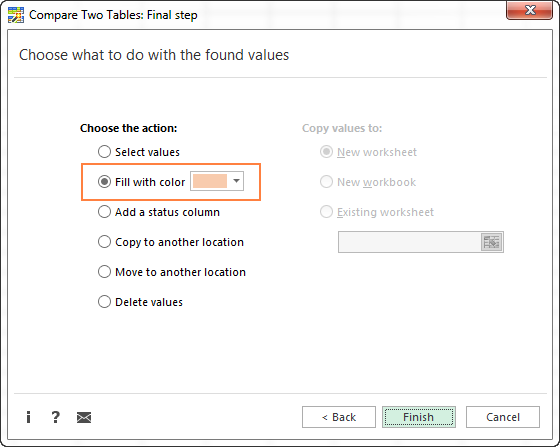
Step 6. In the final step, you choose how to deal with the found items and click Finish.

The following two options deliver the results comparable to Excel formulas and conditional formatting that we've discussed earlier in this tutorial:

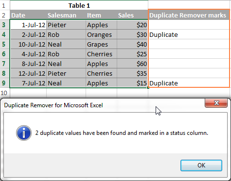
• Add a status column - adds a new column with "Duplicate" or "Unique", like Excel IF formulas do.
• Highlight - shades duplicate or unique rows like an Excel conditional formatting rule.

In addition, you can choose to delete the duplicate entries, move or copy to another worksheet, or just select the found items.

In this example, I've decided to highlight duplicates in the following color:

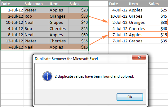
And got the following result in a moment:

If we chose Add a status column in the previous step, the result would look as follows:

This is how you compare and match columns in Excel. If you are interested to try this tool, you are welcome to download a fully functional trial version. And if you like it, we will happily offer you the 15% off coupon code that we've created especially for our blog readers: AB14-BlogSpo. It works both for the Duplicate Remover tool purchased as a separate product and as part of Ultimate Suite for Excel.

If you want to have a closer look at the formulas discussed in this tutorial, feel free to download the Compare Excel Lists workbook. Thank you for reading and see you next week!