Sunday, July 1, 2018

How to compare two columns in Excel for matches and differences

How to compare 2 columns in Excel row-by-row

When you do data analysis in Excel, one of the most frequent tasks is comparing data in each individual row. This task can be done by using the IF function, as demonstrated in the following examples.

Example 1. Compare two columns for matches or differences in the same row

To compare two columns in Excel row-by-row, write a usual IF formula that compares the first two cells. Enter the formula in some other column in the same row, and then copy it down to other cells by dragging the fill handle (a small square in the bottom-right corner of the selected cell). As you do this, the cursor changes to the plus sign:
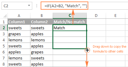
Copy the formula down to other cells to compare two columns in Excel
Formula for matches
To find cells within the same row having the same content, A2 and B2 in this example, the formula is as follows:
=IF(A2=B2,"Match","")
Formula for differences
To find cells in the same row with different content, simply replace "=" with the non-equality sign:
=IF(A2<>B2,"No match","")
Matches and differences
And of course, nothing prevents you from finding both matches and differences with a single formula:
=IF(A2=B2,"Match","No match")
Or
=IF(A2<>B2,"No match","Match")
The result may look similar to this:
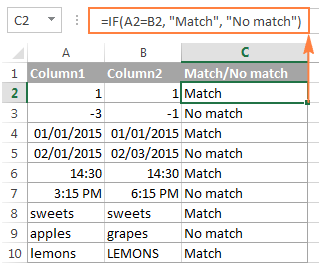
A formula to compare 2 columns for matches and differences in each row
As you see, the formula handles numbersdatestimes and text strings equally well.

Example 2. Compare two lists for case-sensitive matches in the same row

As you have probably noticed, the formulas from the previous example ignore case when comparing text values, as in row 10 in the screenshot above. If you want to find case-sensitive matches between 2 columns in each row, then use the EXACT function:
=IF(EXACT(A2, B2), "Match", "")
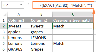
Comparing two lists for case-sensitive matches in the same row
To find case-sensitive differences in the same row, enter the corresponding text ("Unique" in this example) in the 3rd argument of the IF function, e.g.:
=IF(EXACT(A2, B2), "Match", "Unique")

Compare multiple columns for matches in the same row

In your Excel worksheets, multiple columns can be compared based on the following criteria:
  • Find rows with the same values in all columns (Example 1)
  • Find rows with the same values in any 2 columns (Example 2)

Example 1. Find matches in all cells within the same row

If your table has three or more columns and you want to find rows that have the same values in all cells, an IF formula with an AND statement will work a treat:
=IF(AND(A2=B2, A2=C2), "Full match", "")
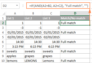
Finding rows that have the same values in all columns
If your table has a lot of columns, a more elegant solution would be using the COUNTIF function:
=IF(COUNTIF($A2:$E2, $A2)=5, "Full match", "")
Where 5 is the number of columns you are comparing.

Example 2. Find matches in any two cells in the same row

If you are looking for a way to compare columns for any two or more cells with the same values within the same row, use an IF formula with an OR statement:
=IF(OR(A2=B2, B2=C2, A2=C2), "Match", "")
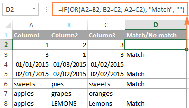
Finding matches in any two cells in the same row
In case there are many columns to compare, your OR statement may grow too big in size. In this case, a better solution would be adding up several COUNTIF functions. The first COUNTIF counts how many columns have the same value as in the 1st column, the second COUNTIF counts how many of the remaining columns are equal to the 2nd column, and so on. If the count is 0, the formula returns "Unique", "Match" otherwise. For example:
=IF(COUNTIF(B2:D2,A2)+COUNTIF(C2:D2,B2)+(C2=D2)=0,"Unique","Match")
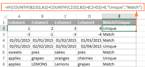
Compare several columns and find matches in any two cells in the same row.

How to compare two columns in Excel for matches and differences

Suppose you have 2 lists of data in Excel, and you want to find all values (numbers, dates or text strings) which are in column A but not in column B.
For this, you can embed the COUNTIF($B:$B, $A2)=0 function in IF's logical test and check if it returns zero (no match is found) or any other number (at least 1 match is found).
For instance, the following IF/COUNTIF formula searches across the entire column B for the value in cell A2. If no match is found, the formula returns "No match in B", an empty string otherwise:
=IF(COUNTIF($B:$B, $A2)=0, "No match in B", "")
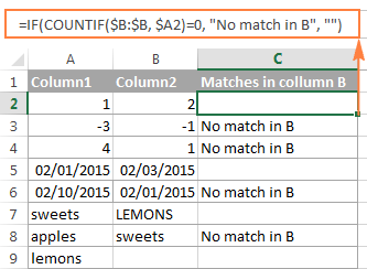
Compare two columns in Excel for matches
Tip. If your table has a fixed number of rows, you can specify a certain range (e.g. $B2:$B10) rather than the entire column ($B:$B) for the formula to work faster on large data sets.
The same result can be achieved by using an IF formula with the embedded ISERROR and MATCH functions:
=IF(ISERROR(MATCH($A2,$B$2:$B$10,0)),"No match in B","")
Or, by using the following array formula (remember to press Ctrl + Shift + Enter to enter it correctly):
=IF(SUM(--($B$2:$B$10=$A2))=0, " No match in B", "")
If you want a single formula to identify both matches (duplicates) and differences (unique values), put some text for matches in the empty double quotes ("") in any of the above formulas. For example:
=IF(COUNTIF($B:$B, $A2)=0, "No match in B", "Match in B")

How to compare two lists in Excel and pull matching data

Sometimes you may need not only match two columns in two different tables, but also pull matching entries from the second table. Microsoft Excel provides a special function for such purposes - the VLOOKUP function. As an alternative, you can use more powerful and versatile INDEX & MATCH formulas.
For example, the following formula compares the product names in columns D and A and if a match is found, a corresponding sales figure is pulled from column B. If no match is found, the #N/A error is returned.
=INDEX($B$2:$B$6,MATCH($D2,$A$2:$A$6,0))
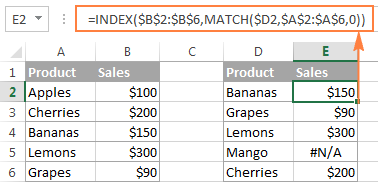
Comparing two lists in Excel and pulling matching data
For the detailed explanation of the formula's syntax and more formula examples, please check out the following tutorial: INDEX & MATCH in Excel - a better alternative to VLOOKUP.
If you don't feel very comfortable with this formula, then you may want to try the Merge Tables wizard - a fast and intuitive solution that can compare and match 2 tables by any column(s).

Compare two lists and highlight matches and differences

When you compare columns in Excel, you may want to "visualize" the items that are present in one column but missing in the other. You can shade such cells in any color of your choosing by using the Excel Conditional Formatting feature and the following examples demonstrate the detailed steps.

Example 1. Highlight matches and differences in each row

To compare two columns and Excel and highlight cells in column A that have identical entries in column B in the same row, do the following:
  • Select the cells you want to highlight (you can select cells within one column or in several columns if you want to highlight entire rows).
  • Click Conditional formatting > New Rule… > Use a formula to determine which cells to format.
  • Create a rule with a simple formula like =$B2=$A2 (assuming that row 2 is the first row with data, not including the column header). Please double check that you use a relative row reference (without the $ sign) like in the formula above.
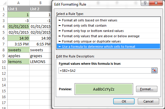
A conditional formatting rule to highlight matches in each row
To highlight differences between column A and B, create a rule with the formula =$B2<>$A2
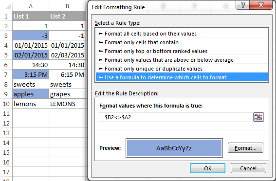
A conditional formatting rule to highlight differences in each row
If you are new to Excel conditional formatting, please see How to create a formula-based conditional formatting rule for step-by-step instructions.

Example 2. Highlight unique entries in each list

Whenever you are comparing two lists in Excel, there are 3 item types that you can highlight:
  • Items that are only in the 1st list (unique)
  • Items that are only in the 2nd list (unique)
  • Items that are in both lists (duplicates) - demonstrated in the next example.
This example demonstrates how to highlight items that are in one list only.
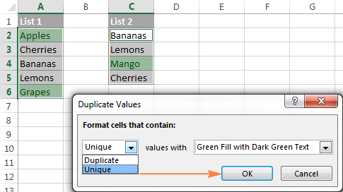
Supposing your List 1 is in column A (A2:A6) and List 2 in column C (C2:C5). You create the conditional formatting rules with the following formulas:
Highlight unique values in List 1 (column A): =COUNTIF($C$2:$C$5, $A2)=0
Highlight unique values in List 2 (column C): =COUNTIF($A$2:$A$6, $C2)=0
And get the following result:
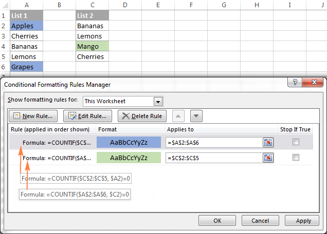
Comparing 2 lists and highlighting unique entries in each list

Example 3. Highlight matches (duplicates) between 2 columns

If you closely followed the previous example, you won't have difficulties adjusting the COUNTIF formulas so that they find the matches rather than differences. All you have to do is to set the count greater than zero:
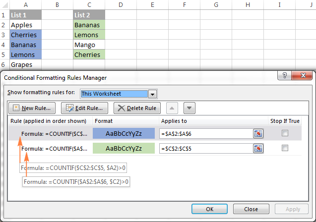
Highlighting matches between 2 columns
Highlight matches in List 1 (column A): =COUNTIF($C$2:$C$5, $A2)>0
Highlight matches in List 2 (column C): =COUNTIF($A$2:$A$6, $C2)>0

Example 4. Built-in rule to compare 2 lists and highlight duplicates or uniques

If you are one of those power users who mostly rely on functions and formulas, you may have missed this amazingly simple way to compare two columns in Excel :)
  • Select two lists you want to compare. If they include different numbers of cells or are located in non-adjacent columns, select the first list, press and hold the Ctrl key, and then select the second list.
  • On the Home tab, go to Conditional Formatting > Highlight Cells Rules > Duplicate Values.
  • Select either Duplicate or Unique from the left-hand side drop-down list, and choose the desired format from the right-hand side drop-down. If you are not happy with any of the predefined formats, click Custom format… and set the Font or Fill color to your liking.
  • Click OK and you are done!
Built-in rule to compare 2 lists and highlight duplicate or unique values

Highlight row differences and matches in multiple columns

When comparing values in several columns row-by-row, the quickest way to highlight matches is creating a conditional formatting rule, and the fastest way to shade differences is embracing the Go To Special feature, as demonstrated in the following examples.

Example 1. Compare multiple columns and highlight row matches

To highlight rows that have identical values in all columns, create a conditional formatting rule based on one of the following formulas:
=AND($A2=$B2, $A2=$C2)
or
=COUNTIF($A2:$C2, $A2)=3
Where A2, B2 and C2 are the top-most cells and 3 is the number of columns to compare.
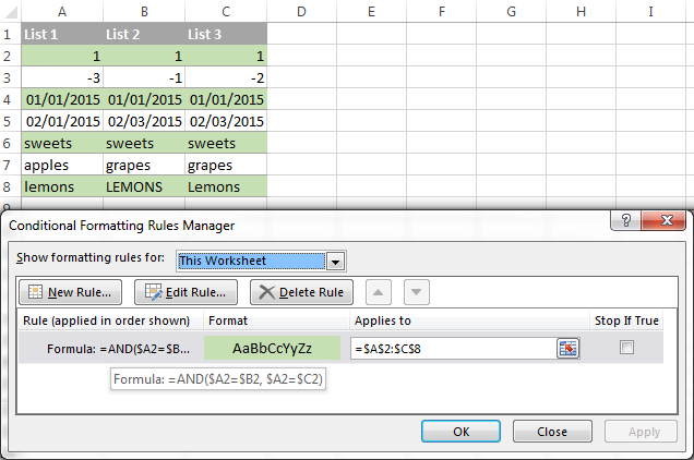
Highlighting rows that have the same values in several columns
Of course, neither AND nor COUNTIF formula is limited to comparing only 3 columns, you can use similar formulas to highlight rows with the same values in 4, 5, 6 or more columns.

Example 2. Compare multiple columns and highlight row differences

To quickly highlight cells with different values in each individual row, you can use Excel's Go To Special feature.
  1. Select the range of cells you want to compare. In this example, I've selected cells A2 to C8.
    Select the range of cells you want to compare.
    By default, the top-most cell of the selected range is the active cell, and the cells from the other selected columns in the same row will be compared to that cell. As you can see in the screenshot above, the active cell is white while all other cells of the selected range are highlighted. In this example, the active cell is A2, so the comparison column is column A.
    To change the comparison column, use either the Tab key to navigate through selected cells from left to right, or the Enter key to move from top to bottom.
    Tip. To select non-adjacent columns, select the first column, press and hold Ctrl, and then select the other columns. The active cell will be in the last column (or in the last block of adjacent columns). To change the comparison column, use the Tab or Enter key as described above.
  2. On the Home tab, go to Editing group, and click Find & Select > Go To Special… Then select Row differences and click the OK button.
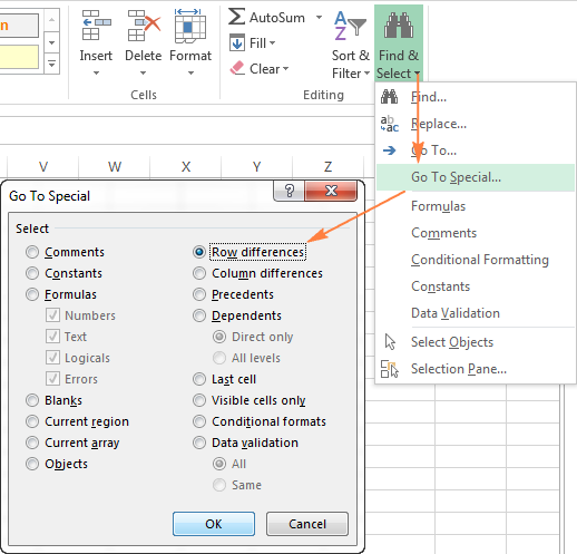
    Select Row differences and click the OK button.
  3. The cells whose values are different from the comparison cell in each row are highlighted.If you want to shade the highlighted cells in some color, simply click the Fill Color icon on the ribbon and select the color of your choosing.
    To shade the highlighted cells in some color, click the Fill Color icon on the ribbon.

How to compare two cells in Excel

In fact, comparing 2 cells is a particular case of comparing two columns in Excel row-by-rowexcept that you don't have to copy the formulas down to other cells in the column.
For example, to compare cells A1 and C1, you can use the following formulas:
For matches: =IF(A1=C1, "Match", "")
For differences: =IF(A1<>C1, "Difference", "")
To learn a few other ways to compare cells in Excel, please see How to compare strings in Excel.
For more powerful data analysis, you may need more sophisticated formulas and you can find a few good ideas in the following tutorials:

Formula-free way to compare two columns / lists in Excel

Now that you know Excel offerings for comparing and matching columns, let me demonstrate you an alternative solution that can compare 2 lists with a different number of columns for matches (duplicates) and differences (unique values).
Ablebits Duplicate Remover for Excel can search for identical and unique entries within one table as well as compare two tables residing on the same sheet or in 2 different worksheets / workbooks.
For the purpose of this article, we will be focusing on the second feature, which is called Compare Two Tables and is specially designed for comparing two lists by any column(s) that you specify. The comparison of two data sets by several columns is a real challenge both for Excel formulas and conditional formatting, but this tool handles it with ease.

Compare 2 lists by several columns in 6 quick steps

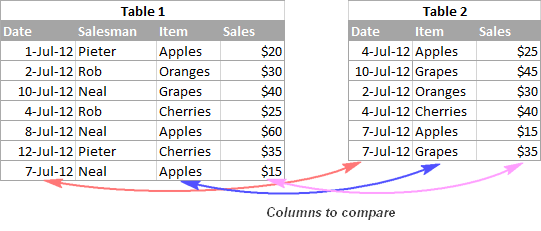
Supposing you have 2 tables of data and you want to find duplicate rows based on 3 columns - DateItem and Sales:
Two tables to be compared by 3 pairs of columns
Step 1. Assuming that you have the Duplicate Remover for Excel installed, select any cell within the 1st table, and click the Compare Two Tables button on the ribbon to start the wizard. This button resides on the Ablebits Data tab, in the Dedupe group.
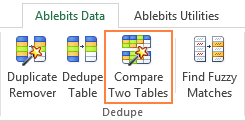
Click the Compare Two Tables button to start the wizard.
Step 2. The wizard picks the entire table and suggests to create a backup copy of the original table, just in case. So, simply make sure your 1st table is selected correctly and click Next.
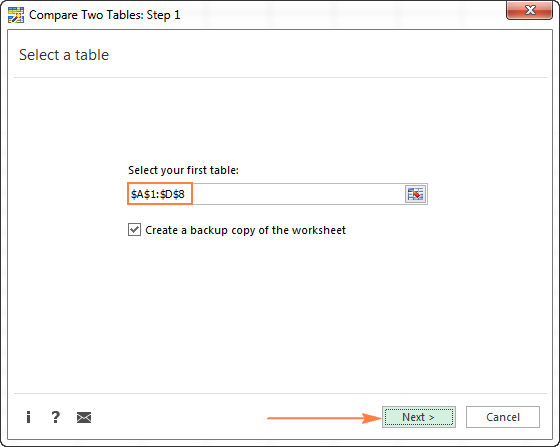
Make sure the first table is selected correctly and click Next.
Step 3. Select the 2nd table by using the standard Select range icon Select range icon. If both tables reside in the same workbook and have similar column names, there's a great chance that the second list will be fetched automatically as well.
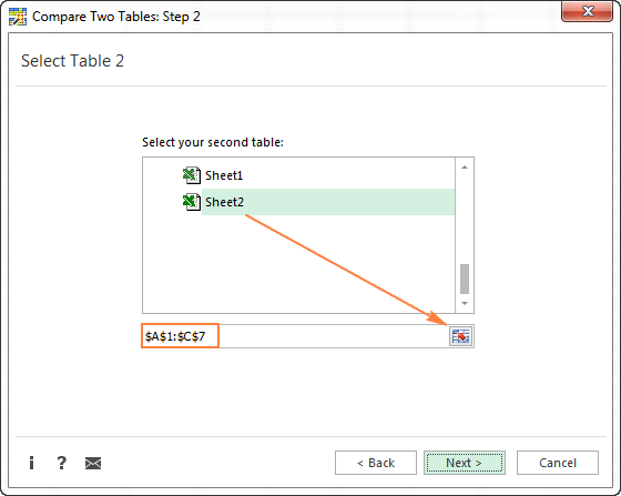
Select the second table to be compared to the first one.
Step 4. Select whether to search for matches or differences:
  • Duplicate values - look for matches, i.e. items that exist in both tables.
  • Unique values - look for differences, i.e. items that are in Table 1 but not in Table 2.
In this example, we select Duplicate values and click Next.
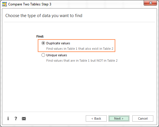
Select whether to search for matches or differences.
Step 5. This is the key step where you select the column pairs you want to compare in 2 tables. In this example, we are comparing 3 columns - DateItem and Sales.
For the wizard to find the matching columns automatically, click the Auto Detect button in the upper-right corner. If the columns have different names in both tables, you might need to select the right column manually by clicking the little black arrow next to the Table 2 column on the right-hand side:
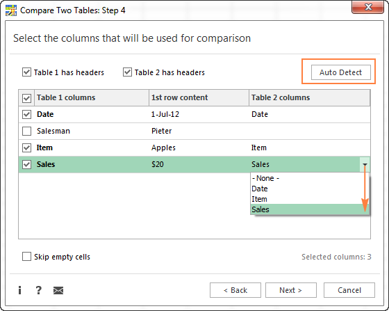
Select the pairs of columns to be compared in 2 tables.
Step 6. In the final step, you choose how to deal with the found items and click Finish.
The following two options deliver the results comparable to Excel formulas and conditional formatting that we've discussed earlier in this tutorial:
  • Add a status column - adds a new column with "Duplicate" or "Unique", like Excel IF formulas do.
  • Highlight - shades duplicate or unique rows like an Excel conditional formatting rule.
In addition, you can choose to delete the duplicate entries, move or copy to another worksheet, or just select the found items.
In this example, I've decided to highlight duplicates in the following color:
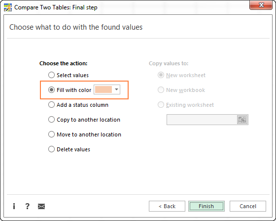
Choose how to deal with the found duplicate items.
And got the following result in a moment:
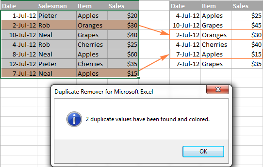
Duplicate rows are highlighted.
If we chose Add a status column in the previous step, the result would look as follows:
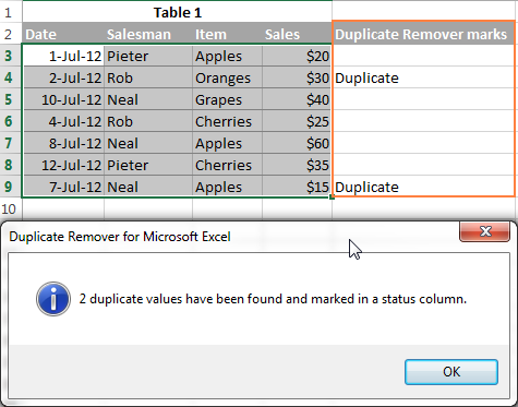
Duplicate rows are marked.
This is how you compare and match columns in Excel. If you are interested to try this tool, you are welcome to download a fully functional trial version. And if you like it, we will happily offer you the 15% off coupon code that we've created especially for our blog readers: AB14-BlogSpo. It works both for the Duplicate Remover tool purchased as a separate product and as part of Ultimate Suite for Excel.
If you want to have a closer look at the formulas discussed in this tutorial, feel free to download the Compare Excel Lists workbook. Thank you for reading and see you next week!

Saturday, June 30, 2018

How to Install Adobe Photoshop CS5 Full Version

If you’re looking for an image editing suite it will not matter whether you’re using Windows or Mac OS on a 32 bit machine or a 64 bit machine, Adobe Photoshop will be your first choice. Photoshop is such a powerful program that even older versions of the program can match most tasks. Adobe Photoshop CS5 was released in 2010 meaning people having been running it on old operating systems like Windows XP, Windows 7 and Windows 8 for years. Despite its age, however, it is still a really powerful piece of software so it is definitely worth knowing How to Download Adobe Photoshop CS5.
How to Download Adobe Photoshop cs5
These days Adobe run a subscription based service meaning there is no real need to buy the program outright or for an installer or a setup exe file. Also there are new procedures to follow regarding how to obtain and how to use serial numbers.

Why Install Adobe Photoshop CS5 Free Full Version?

A free download of a full version of Adobe Photoshop CS5 gives you access to a plethora of cool Photoshop features. CS5 has a number of great features and tools including:
  • Content-Aware Fill
  • Refine Edge
  • Mixer Brush
  • Bristle Tips
  • Puppet Warp
Other community led additions to Photoshop CS5 included:
  • Automatic image straightening,
  • The Rule-of-Thirds cropping tool,
  • Color pickup
  • 16-bit image saves as a JPEGs.
Also, for ease of use via improved file management and browsing Adobe Photoshop CS5 also includes the Adobe Mini Bridge, which allows for seamless file management and browsing.

How to Download Adobe Photoshop cs5

Adobe Photoshop CS5 System Requirements

Windows
  • Intel® Pentium® 4 or AMD Athlon® 64 processor
  • Microsoft® Windows® XP with Service Pack 3; Windows Vista® Home Premium, Business, Ultimate, or Enterprise with Service Pack 1 (Service Pack 2 recommended); or Windows 7
  • 1 GB of RAM
  • 1 GB of available hard-disk space for installation; additional free space required during installation (cannot install on removable flash-based storage devices)
  • 1024 x 768 display (1280 x 800 recommended) with qualified hardware-accelerated OpenGL graphics adapter, 16-bit color, and 256 MB of VRAM
  • Some GPU-accelerated features require graphics support for Shader Model 3.0 and OpenGL 2.0
  • DVD-ROM drive
  • QuickTime 7.6.2 software required for multimedia features
Mac OS

  • Multicore Intel processor
  • Mac OS X v10.5.7 or v10.6
  • 1 GB of RAM
  • 2 GB of available hard-disk space for installation; additional free space required during installation (cannot install on a volume that uses a case-sensitive file system or on removable flash-based storage devices)
  • 1024 x 768 display (1280 x 800 recommended) with qualified hardware-accelerated OpenGL graphics adapter, 16-bit color, and 256 MB of VRAM
  • Some GPU-accelerated features require graphics support for Shader Model 3.0 and OpenGL 2.0
  • DVD-ROM drive
  • QuickTime 7.6.2 software required for multimedia features

How to Install Adobe Photoshop CS6 Full Version

How to Install Adobe Photoshop CS6 Full Version

If you have arrived here that means that you are looking for an image editing suite. We are sure that there’s 99% chance that you were looking to download a free full version of the great Adobe Photoshop CS6. And we understand that. Adobe Photoshop is the clear choice when you want an image editing suite, no matter if you are using Windows or Mac OS or if you have a 32 bit machine or a 64 bit machine. The bad news is that Adobe Photoshop CS6 was released back in 2012 and it runs on old systems such as Windows XP, Windows 7, Windows 8 and Mac OS X v10.6.8. You won’t find Adobe Photoshop CS5 anymore. At least not legally.
button_get-the-adobe-photoshop-cc-latest-version
Don’t worry. Adobe is still going it is just that nowadays it runs as a subscription based service. This means that you don’t need to buy the program anymore and you don’t need an installer or a setup exe file. This also means that you’ll always have the most advanced Adobe Photoshop version ready for your service.

×

Was it Worth it to Download and Install Adobe Photoshop CS6 Full Version?

A download of the full version of Adobe Photoshop CS6 gives you access to a plethora of cool Photoshop features. CS6 has a number of great features and tools including:
  • Content-Aware Patch
  • Adobe Mercury Graphics Engine
  • New and Re-engineered Design Tools
  • Intuitive Video Creation
  • Blur Gallery
Post-launch patches included additions to Photoshop CS6 such as:
  • Vector Shapes
  • Updated User Interface
  • “Liquify” filter
  • Layer styles/Blending Options dialog
Also, the Adobe Photoshop CS6 Extended version included exclusive features like the Mercury Graphics Engine, which is a powerful engine for optimizing 3D imagery; new controls for more efficient 3D workflows and new effects such as reflections and dragable shadows.
So, was it worth it to download Adobe CS6? Yes, yes and ten thousand times yes.

button_get-the-adobe-photoshop-cc-latest-version

Adobe Photoshop CS6 System Requirements

Windows
  • Intel® Pentium® 4 or AMD Athlon® 64 processor
  • Microsoft® Windows® XP with Service Pack 3 orMicrosoft Windows 7 with Service Pack 1. Adobe® Creative Suite® 5.5 and CS6 applications also support Windows 8 and Windows 8.1. See the CS6 FAQ for more information about Windows 8 support
  • 1 GB of RAM
  • 1 GB of available hard-disk space for installation; additional free space required during installation (cannot install on removable flash-based storage devices)
  • 1024 x 768 display (1280 x 800 recommended) with 16-bit color and 512 MB (1 GB recommended) of VRAM
  • OpenGL 2.0–capable system
  • DVD-ROM drive
  • This software doesn’t operate without activation. Broadband Internet connection and registration are required for software activation, validation of subscriptions, and access to online service
Mac OS
  • Multicore Intel processor with 64-bit support
  • Mac OS X v10.6.8 or v10.7. Adobe Creative Suite 3, 4, 5, CS5.5, and CS6 applications support Mac OS X v10.8 or v10.9 when installed on Intel-based systems
  • 1 GB of RAM
  • 2 GB of available hard-disk space for installation; additional free space required during installation (cannot install on a volume that uses a case-sensitive file system or on removable flash-based storage devices)
  • 1024 x 768 display (1280 x 800 recommended) with 16-bit color and 512 MB (1 GB recommended) of VRAM
  • OpenGL 2.0–capable system
  • DVD-ROM drive
  • This software doesn’t operate without activation. Broadband Internet connection and registration are required for software activation, validation of subscriptions, and access to online service

Adobe Photoshop 7.0.1 Update


Essential update for Adobe Photoshop 7.0.1


Friday, June 29, 2018

Use the PROPER function to capitalize names in Excel


When you think about Excel functions, you probably think about performing calculations with numbers. While it's true that you can use functions to do lots of handy things with numbers in Excel, some functions can help you format text too. One good example is the PROPER function, which capitalizes the first letter of every wordin a cell. If you have cells containing proper nouns, like names or titles, you can use the PROPER function to make sure everything is capitalized correctly. The PROPER function works in Google Sheets too.
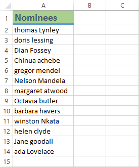
For example, let's say your company wants to give someone a lifetime achievement award. You've asked your coworkers to enter their nominations for the award into this spreadsheet:
screenshot of Microsoft Excel
Unfortunately, you can see that not everyone has been careful to capitalize the first and last names of the people they want to nominate, so the spreadsheet looks messy. You could go through the column and correct the names manually, but using the PROPER function will be faster and easier.
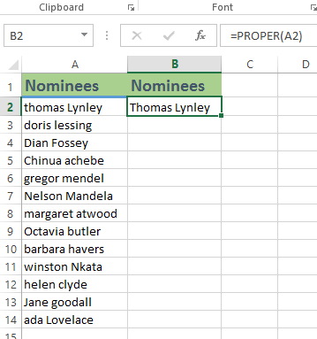
In this example, the names of the nominees are in column A, so we'll put our formula in column B. In cell B2, we'll type a formula that tells Excel to capitalize the name in cell A2, which contains the first name on our list. The formula will look like this:
=PROPER(A2)
As you may remember from our Simple Formulas lesson in our Excel Formulastutorial, it's important to make sure you start any Excel formula with an equals sign. Once you've entered the formula, press the Enter key, and cell B2 will display the name from A2 with the correct capitalization: Thomas Lynley.
screenshot of Microsoft Excel
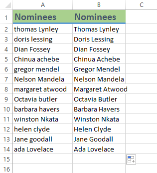
Now all we have to do is click and drag the fill handle through cell A14, and column B will display all of the names in the list with the correct capitalization:
screenshot of Microsoft Excel
Great! Now all the names of the award nominees are correctly capitalized in the spreadsheet. There's one problem, though: We still have the original uncapitalized names in column A. We can't delete column A because our formula in column B refers to it. Instead, we can copy the values from column B into a new column by using the Paste Values feature in Excel.
To do this, select cells B2:B14 and click the Copy command (or press Ctrl+C on your keyboard). Then right-click the cell where you want to paste the values (C2, for example), then select the Values button from the menu that appears. If you're using Google Sheets, you can right-click and go to Paste special > Paste values only.
screenshot of Microsoft Excel
Now we have a column that displays the corrected names but that doesn't depend on a formula or cell reference. This means we can delete our original columns (column A and column B). There we have it: a nice, neat spreadsheet with all the names of the nominees correctly capitalized.

CONCATENATE: Excel's duct tape

MacGyver used it. The Apollo 13 crew used it. Whenever people are in a bind and need to stick two things together, they reach for the duct tape. But what you may not know is that Excel has a built-in function that does pretty much the same thing: CONCATENATE.
CONCATENATE lets you combine two or more things in one cell—and despite the long name, it's actually easy to use. It works the same way in all versions of Excel, as well as in other spreadsheet applications like Google Sheets.
If you'd like to follow along, you can download our example spreadsheet. Note: If you've never used Excel functions before, you may want to check out our Functionslesson from our Excel Formulas tutorial first to learn the basics.

Combining names

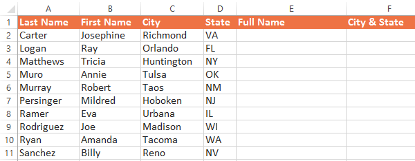
Let's say we have a spreadsheet of contact information with last names and first names in separate columns, and we'd like to combine them to get each person's full name. In the image below, you can see that the first names are in column B and the last names are in column A. Our formula will go in cell E2.
screenshot of Microsoft Excel
Before we start typing the formula, there's one important thing you need to know: CONCATENATE will combine exactly what you tell it to combine, and nothing more.If you want punctuation, spaces, or any other details to appear in the cell, you'll need to tell CONCATENATE to include it. In this case, we want the names to have a space in between them (so it doesn't say JosephineCarter), so we'll need to add an argument that contains a space. This means we'll need three arguments:
  • B2 (first name)
  • " " (a space in quotation marks)
  • A2 (last name)
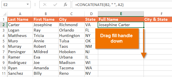
Now that we have our arguments, we can type the following formula into cell E2:
=CONCATENATE(B2, “ ”, A2)
Just like any function, the syntax is important. Make sure to start with an equals sign, and separate each argument with a comma. Note: Depending on where you live, you may need to separate the arguments with a semicolon (;) instead of a comma.
That's it! When you press Enter, it should display the full name: Josephine Carter.
Now you can click and drag the fill handle down through cell E11, and it should display the full name for each person.
screenshot of Microsoft Excel
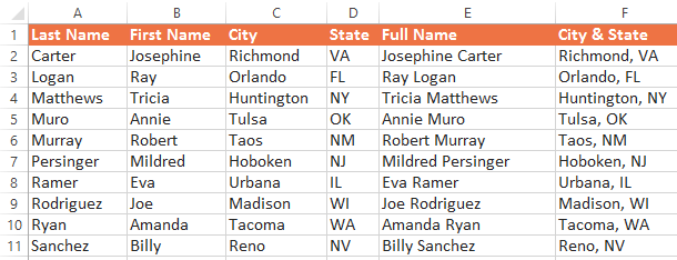
If you'd like an extra challenge, try using CONCATENATE to combine the city and statein column F so it looks like the image below.
screenshot of Microsoft Excel

Combining numbers and text

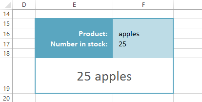
You can even use CONCATENATE to combine numbers and text. For example, let's say we're using Excel to keep track of a store's inventory. We currently have 25 apples in stock, but 25 and apples are in separate cells. We want to combine them into one cell so that it looks like this:
screenshot of Microsoft Excel
To do this, we'll need to combine three things:
  • F17 (number in stock)
  • " " (space)
  • F16 (product name)
Type the following formula into cell E19:
=CONCATENATE(F17, “ ”, F16)
Let's say we want it to say We have 25 apples. We'll just need to add an argument at the beginning that says We have:
=CONCATENATE(“We have ”, F17, “ ”, F16)
If you wanted to, you could add even more arguments to create more complex statements. Just keep in mind that the syntax always needs to be exactly right, or the formula may not work—and it's easier to make a mistake with a longer formula.

Use SUMPRODUCT to calculate weighted averages


Excel makes it extremely easy to calculate the average of several cells: Just use the AVERAGE function. But what if some of the values have more "weight" than others? For example, in many classes the tests are worth more than the assignments. For these situations, you'll need to calculate the weighted average.
Although Excel doesn't have a weighted average function, it does have a function that does most of the work for you: SUMPRODUCT. Even if you've never used SUMPRODUCT before, you'll be able to use it like a pro by the end of this article. The method we're using works with all versions of Excel, and it also works with other spreadsheet applications like Google Sheets.
If you'd like to follow along, you can download our example.

Setting up the spreadsheet

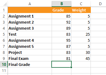
In order to calculate the weighted average, you'll need at least two columns. The first column (column B in our example) contains the grades for each assignment or test. The second column (column C) contains the weights. A higher weight will cause the assignment or test to have a greater effect on the final grade.
You can think of the weight as being the percentage of the final grade. But in this case, the weights actually add up to more than 100%. That's OK because our formula will still work no matter what the weights add up to.
screenshot of Microsoft Excel

Entering the formula

Now that we have our spreadsheet set up, we'll add the formula to cell B10 (any empty cell will work). As with any formula, start by typing an equals sign (=).
The first part of our formula will be the SUMPRODUCT function. Because the arguments will be in parentheses, go ahead and type an open parenthesis:
=SUMPRODUCT(
Next, we'll add the arguments to the function. SUMPRODUCT can have any number of arguments, but it will usually have two. In our example, the first argument will be the cell range B2:B9—the cells that contain our grades:
=SUMPRODUCT(B2:B9
The second argument will be the cell range C2:C9—the cells that contain the weights. You'll need to use a comma to separate these two arguments. When you're done, type a closed parenthesis:
=SUMPRODUCT(B2:B9, C2:C9)
Now we'll add the second part of our formula. This part will divide SUMPRODUCT by the SUM of the weights. Later, we'll talk about why this is important.
Start by typing a / (forward slash) for division, and then type the SUM function:
=SUMPRODUCT(B2:B9, C2:C9)/SUM(
We just need one argument for the SUM function: the cell range C2:C9. Remember to close the parentheses after the argument:
=SUMPRODUCT(B2:B9, C2:C9)/SUM(C2:C9)
That's it! When you press Enter on your keyboard, Excel will calculate the weighted average. In our example, the final grade is 83.6.

How it works

Let's look at each part of this formula to see how it works, starting with the SUMPRODUCT function. SUMPRODUCT is multiplying (finding the product of) each assignment's grade times its weight, then adding all of the products together. In other words, it finds the sum of the products, which is where it gets its name. So for Assignment 1 it multiplies 85 by 5, and for the Test it multiplies 83 by 25.
If you're wondering why the values needed to be multiplied in the first place, think of it this way: The assignments with a higher weight are counted more times. For example, Assignment 2 is counted 5 times, but the Final Exam is counted 45 times. This is why the Final Exam has a bigger impact on the final grade. By comparison, a "regular" average would count each assignment one time, so each one has the same weight.
If you could look "under the hood" of the SUMPRODUCT function, you would see that this is what it is actually calculating:
=(B2*C2)+(B3*C3)+(B4*C4)+(B5*C5)+(B6*C6)+(B7*C7)+(B8*C8)+(B9*C9)
Luckily, we don't have to write a long formula like this because SUMPRODUCT is doing all of it automatically.
By itself, SUMPRODUCT will give us a huge number: 10,450. This is where the second part of our formula comes in: /SUM(C2:C9). This part brings the value back down to a normal grade range, making the answer 83.6.
The second part of the formula is actually really useful because it allows the formula to automatically correct its calculations. Remember that the weights don't need to add up to 100%? This is because this part of the formula takes care of that for us. For example, if we increase one or more of the weights, the second part of the formula simply divides by a higher number, bringing it back down to the correct answer. We could even make the weights much smaller, giving them values like 0.5, 2.5, 3.0, and 4.5, and the formula would still work perfectly. Pretty neat, huh?