In this tutorial, we will be looking at how to use IFERROR and VLOOKUP functions together to trap and handle different errors. In addition, you are going to learn how to do sequential vlookups in Excel by nesting multiple IFERROR functions one onto another.
Excel VLOOKUP and IFERROR - these two functions may be pretty hard to understand separately, let alone when they are combined. In this article, you will find a few easy-to-follow examples that address common uses and clearly illustrate the formulas' logic.
If you don't have much experience with IFERROR and VLOOKUP functions, it may be a good idea to revise their basics first by following the above links.
IFERROR with VLOOKUP to handle #N/A and other errors
When Excel Vlookup fails to find a lookup value, it throws an #N/A error, like this:
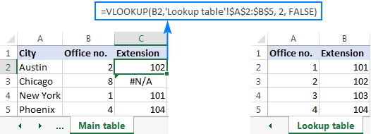

Depending on your business needs, you may want to disguise the error with your own text, zero, or a blank cell.
Example 1. Iferror Vlookup formula to replace all errors with your own text
If you'd like to replace the standard error notation with your custom text, wrap your Vlookup formula in IFERROR, and type any text you want in the 2nd argument (value_if_error), for example "Not found":
IFERROR(VLOOKUP(…),"Not found")
With the lookup value in B2 in the Main table and the lookup range A2:B4 in the Lookup table, the formula takes the following shape:
=IFERROR(VLOOKUP(B2,'Lookup table'!$A$2:$B$5, 2, FALSE), "Not found")
The screenshot below shows our Excel IFERROR VLOOKUP formula in action:
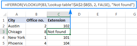

The result looks much more understandable and far less intimidating, isn't it?
In a similar manner, you can use INDEX MATCH together with IFERROR:
=IFERROR(INDEX('Lookup table'!$B$2:$B$5,MATCH(B2,'Lookup table'!$A$2:$A$5,0)), "Not found")
The IFERROR INDEX MATCH formula is especially useful when you want to pull values from a column that lies to the left of the lookup column (left lookup), and return your own text when nothing is found.
Example 2. Iferror with Vlookup to return blank or 0 if nothing is found
If you don't want to show anything when the lookup value is not found, have IFERROR display an empty string (""):
IFERROR(VLOOKUP(…),"")
In our example, the formula goes as follows:
=IFERROR(VLOOKUP(B2,'Lookup table'!$A$2:$B$5, 2, FALSE), "")
As you can see, it returns nothing when the lookup value is not in the search list.
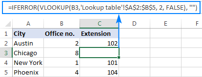

If you'd like to replace the error with the zero value, put 0 in the last argument:
=IFERROR(VLOOKUP(B2,'Lookup table'!$A$2:$B$5, 2, FALSE), 0)
Word of caution! Excel IFERROR function catches all kinds of errors, not only #N/A. Is it good or bad? All depends on your goal. If you want to mask all possible errors, IFERROR Vlookup is the way to go. But it may be an unwise technique in many situations.
For example, if you've created a named range for your table data, and misspelled that name in your Vlookup formula, IFERROR will catch a #NAME? error and replace it with "Not found" or any other text you supply. As the result, you may never know your formula is delivering wrong results unless you spot the typo yourself. In such a case, a more reasonable approach would be trapping only #N/A errors. For this, use IFNA Vlookup formula in Excel 2016 and Excel 2013, IF ISNA VLOOKUP in all Excel versions.
The bottom line is: be very careful when choosing a companion for your Vlookup formula :)
Nest IFERROR within VLOOKUP to always find something
Imagine the following situation: you look up a specific value in a list and do not find it. What choices do you have? Either get an N/A error or show your own message. Actually, there is a third option - if your primary vlookup stumbles, then search for something else that is definitely there!
Taking our example further, let's create some sort of dashboard for our users that will show them an extension number of a specific office. Something like this:
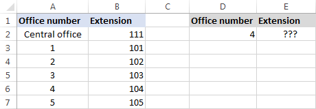

So, how do you pull the extension from column B based on the office number in D2? With this regular Vlookup formula:
=VLOOKUP($D$2,$A$2:$B$7,2,FALSE)
And it will work nicely as long as your users enter a valid number in D2. But what if a user inputs some number that does not exist? In this case, let them call the central office! For this, you embed the above formula in the value argument of IFERROR, and put another Vlookup in the value_if_errorargument.
The complete formula is a bit long, but it works perfectly:
=IFERROR(VLOOKUP("office "&$D$2,$A$2:$B$7,2,FALSE),VLOOKUP("central office",$A$2:$B$7,2,FALSE))
If the office number is found, the user gets the corresponding extension number:


If the office number is not found, the central office extension is displayed:


To make the formula a bit more compact, you can use a different approach:
First, check if the number in D2 is present in the lookup column (please notice that we set col_index_num to 1 for the formula to look up and return value from column A): VLOOKUP(D2,$A$2:$B$7,1,FALSE)
If the specified office number is not found, then we search for the string "central office", which is definitely in the lookup list. For this, you wrap the first vlookup in IFERROR and nest this whole combination inside another Vlookup function:
=VLOOKUP(IFERROR(VLOOKUP(D2,$A$2:$B$7,1,FALSE),"central office"),$A$2:$B$7,2)
Well, a slightly different formula, the same result:
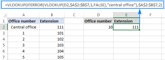

But what is the reason to look up "central office", you may ask me. Why not supply the extension number directly in IFERROR? Because the extension may change at some point in the future. If this happens, you will have to update your data just once in the source table, without worrying about updating each of your Vlookup formulas.
How to do sequential Vlookups in Excel
In situations when you need to perform multiple Vlookups in Excel depending on whether a prior Vlookup succeeded or failed, nest two or more IFERROR functions to evaluate multiple conditions one by one:
IFERROR(VLOOKUP(…), IFERROR(VLOOKUP(…), IFERROR(VLOOKUP(…),"Not found")))
The formula works with the following logic:
If the first Vlookup does not find anything, the first IFERROR traps an error and runs another Vlookup. If the second Vlookup fails, the second IFERROR catches an error and runs the third Vlookup, and so on. If all vlookups stumble, the last IFERROR returns your message.
This nested IFERROR formula is especially useful when you have to search through multiple sheets as shown in the below example.
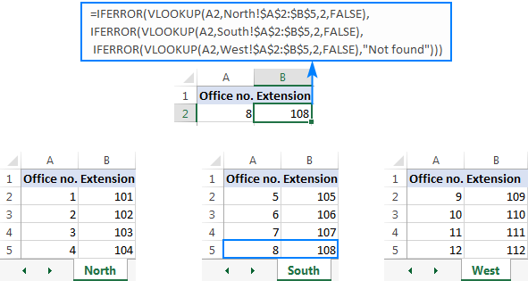
Let's say, you have three lists of homogeneous data in three different worksheets (office numbers in this example), and you want to get an extension for a certain number.
Assuming the lookup value is in cell A2 in the current sheet, and the lookup range is A2:B5 in 3 different worksheets (North, South and West), the following formula works a treat:
=IFERROR(VLOOKUP(A2,North!$A$2:$B$5,2,FALSE), IFERROR(VLOOKUP(A2,South!$A$2:$B$5,2,FALSE), IFERROR(VLOOKUP(A2,West!$A$2:$B$5,2,FALSE),"Not found")))
So, our "chained Vlookups" formula searches in all three sheets in the order we nested them in the formula, and brings the first match it finds:

This is how you use IFERROR with VLOOKUP in Excel. To have a closer look at the formulas discussed in this tutorial, please feel free to download our sample Excel Iferror Vlookupworkbook. I thank you for reading and hope to see you on our blog next week!


0 comments:
Post a Comment