How to use VLOOKUP & SUM or SUMIF functions in Excel

In this tutorial, you will find a handful of advanced formula examples that demonstrate how to use Excel's VLOOKUP and SUM or SUMIF functions to look up and sum values based on one or several criteria.

Are you trying to create a summary file in Excel that will identify all instances of one particular value, and then sum other values that are associated with those instances? Or, do you need to find all values in an array that meet the condition you specify and then sum the related values from another worksheet? Or maybe you are faced with a more concrete challenge, like looking through a table of your company invoices, identifying all invoices of a particular vendor, and then summing all the invoice values?

The tasks may vary, but the essence is the same - you want to look up and sum values with one or several criteria in Excel. What kind of values? Any numeric values. What sort of criteria? Any : ) Starting from a number or reference to a cell containing the right value, and ending with logical operators and results returned by Excel formulas.

So, does Microsoft Excel have any functionality that can help with the above tasks? Of course, it does! You can work out a solution by combining Excel's VLOOKUP or LOOKUP with SUM or SUMIF functions. The formula examples that follow below will help you understand how these Excel functions work and how to apply them to real data.

Please note, these are advanced examples that imply you are familiar with the general principles and syntax of the VLOOKUP function. If not, the first part of our VLOOKUP tutorial for beginners is certainly worth your attention - Excel VLOOKUP syntax and general usages.

• VLOOKUP and SUM - sum all matching values
• Other calculations with VLOOKUP (AVERAGE, MAX, MIN)
• LOOKUP AND SUM - look up in array and sum associated values
• VLOOKUP and SUMIF - sum values that meet certain criteria
• Formula-free way to do vlookup in Excel

Excel VLOOKUP and SUM - find the sum of matching values

If you work with numerical data in Excel, quite often you have not just to extract associated values from another table but also sum numbers in several columns or rows. To do this, you can use a combination of the SUM and VLOOKUP functions as demonstrated below.

Suppose, you have a product list with sales figures for several months, a column per each month.

Source data - Monthly Sales:

Now, you want to make a summary table with the total sales for each product.

The solution is to use an array in the 3^rd parameter (col_index_num) of the Excel VLOOKUP function. Here is a sample VLOOKUP formula:

=SUM(VLOOKUP(lookup value, lookup range, {2,3,4}, FALSE))

As you see, we use an array {2,3,4} in the third argument to perform several lookups within the same VLOOKUP formula in order to get the sum of values in columns 2,3 and 4.

And now, let's adjust this combination of VLOOKUP and SUM functions for our data to find the total of sales in columns B - M in the above table:

=SUM(VLOOKUP(B2, 'Monthly sales'! $A$2:$M$9, {2,3,4,5,6,7,8,9,10,11,12,13}, FALSE))

Important! Since you are building an array formula, be sure to hit Ctrl + Shift + Enter instead of a simple Enter keystroke when you finished typing. When you do this, Microsoft Excel encloses your formula in curly braces like this:

{=SUM(VLOOKUP(B2, 'Monthly sales'!$A$2:$M$9, {2,3,4,5,6,7,8,9,10,11,12,13}, FALSE))}

If you press the Enter key as usual, only the first value in the array will get processed, which will produce incorrect results.

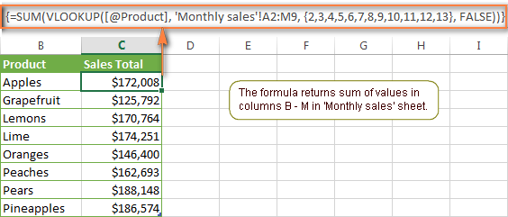
Tip. You may be curious why the formula displays [@Product] as the lookup value in the screenshot above. This is because I converted my data to table (Insert tab > Table). I find it very convenient to work with fully-functional Excel tables rather than mere ranges. For example, when you type a formula into one cell, Excel automatically copies it across the entire column and in this way saves you a few precious seconds :)

As you see, using the VLOOKUP and SUM functions in Excel is easy. However, this is not the ideal solution, especially if you are working with big tables. The point is that using array formulas may adversely affect the workbook's performance since each value in the array makes a separate call of the VLOOKUP function. So, the more values you have in the array and the more array formulas you have in your workbook, the slower Excel works.

You can bypass this problem by using a combination of the INDEX and MATCH functions instead of SUM and VLOOKUP, and I will show you a few formula examples in the next article.

Download this VLOOKUP and SUM sample.

How to perform other calculations with Excel VLOOKUP function

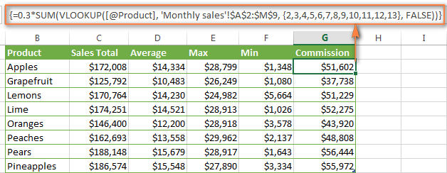
A moment ago we discussed an example of how you can extract values from several columns in the lookup table and calculate the sum of those values. In the same fashion, you can perform other mathematical calculations with the results returned by the VLOOKUP function. Here are a few formula examples:

Operation	Formula example	Description
Calculate average	{=AVERAGE(VLOOKUP(A2, 'Lookup Table'$A$2:$D$10, {2,3,4}, FALSE))}	The formula searches for the value of cell A2 in 'Lookup table' and calculates the average of values in columns B,C and D in the same row.
Find maximum value	{=MAX(VLOOKUP(A2, 'Lookup Table'$A$2:$D$10, {2,3,4}, FALSE))}	The formula searches for the value of cell A2 in 'Lookup table' and finds the max value in columns B,C and D in the same row.
Find minimum value	{=MIN(VLOOKUP(A2, 'Lookup Table'$A$2:$D$10, {2,3,4}, FALSE))}	The formula searches for the value of cell A2 in 'Lookup table' and finds the min value in columns B,C and D in the same row.
Calculate % of sum	{=0.3*SUM(VLOOKUP(A2, 'Lookup Table'$A$2:$D$10, {2,3,4}, FALSE))}	The formula searches for the value of cell A2 in 'Lookup table', sums values in columns B,C and D in the same row, and then calculates 30% of the sum.

Note. Since all of the above formulas are array formulas, remember to press Ctrl+Shift+Enterto enter them correctly in a cell.

If we add the above formulas to the 'Summary Sales' table from the previous example, the result will look similar to this:

Download this VLOOKUP calculations sample.

LOOKUP AND SUM - look up in array and sum matching values

In case your lookup parameter is an array rather than a single value, the VLOOKUP function is of no avail because it cannot look up in data arrays. In this case, you can use Excel's LOOKUP function that is analogues to VLOOKUP but works with arrays as well as with individual values.

Let's consider the following example, so that you can better understand what I'm talking about. Suppose, you have a table that lists customer names, purchased products and quantity (Main table). You also have a second table containing the product prices (Lookup table). Your task is to make a formula that finds the total of all orders made by a given customer.

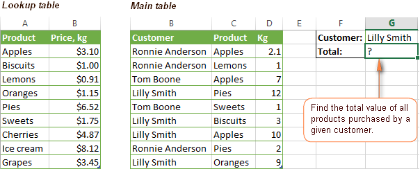
As you remember, you cannot utilize the Excel VLOOKUP function since you have multiple instances of the lookup value (array of data). Instead, you use a combination of SUM and LOOKUP functions like this:

=SUM(LOOKUP($C$2:$C$10,'Lookup table'!$A$2:$A$16,'Lookup table'!$B$2:$B$16)*$D$2:$D$10*($B$2:$B$10=$G$1))

Since this is an array formula, remember to press Ctrl + Shift + Enter to complete it.

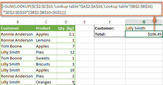
And now, let's analyses the formula's ingredients so that you understand how each of the functions works and can to tweak it for your own data.

We'll put aside the SUM function for a while, because its purpose is obvious, and focus on the 3 components that are multiplied:

1. LOOKUP($C$2:$C$10,'Lookup table'!$A$2:$A$16,'Lookup table'!$B$2:$B$16)
   This LOOKUP function looks up the goods listed in column C in the main table, and returns the corresponding price from column B in the lookup table.
2. $D$2:$D$10
   This component returns quantity of each product purchased by each customer, which is listed in column D in the main table. Multiplied by the price, which is returned by the LOOKUP function above, it gives you the cost of each purchased product.
3. $B$2:$B$10=$G$1
   This formula compares the customers' names in column B with the name in cell G1. If a match is found, it returns "1", otherwise "0". You use it simply to "cut off" customers' names other than the name in cell G1, since all of us know that any number multiplied by zero is zero.

Because our formula is an array formula it iterates the process described above for each value in the lookup array. And finally, the SUM function sums the products of all multiplications. Nothing difficult at all, it is?

Note. For the LOOKUP formula to work correctly you need to sort the lookup column in your Lookup table in ascending order (from A to Z). If sorting is not acceptable on your data, check out an awesome SUM / TRANSPOSE formula suggested by Leo.

Download this LOOKUP and SUM sample.

VLOOKUP and SUMIF - look up & sum values that meet certain criteria

Excel's SUMIF function is similar to SUM we've just discussed in the way that it also sums values. The difference is that the SUMIF function sums only those values that meet the criteria you specify. For example, the simplest SUMIF formula =SUMIF(A2:A10,">10") adds the values in cells A2 to A10 that are larger than 10.

This is very easy, right? And now let's consider a bit more complex scenario. Suppose you have a table that lists the sales persons' names and ID numbers (lookup table). You have another table that contains the same IDs and associated sales figures (main table). Your task is to find the total of sales made by a given person by their ID. At that, there are 2 complicating factors:

• The mail table contains multiple entries for the same ID in a random order.
• You cannot add the "Sales person names" column to the main table.

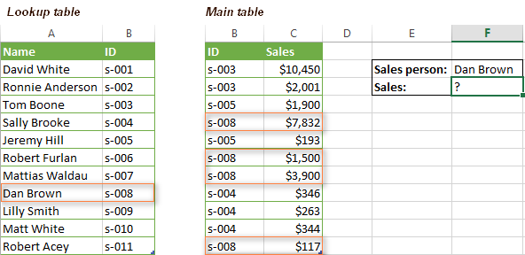
And now, let's make a formula that, firstly, finds all sales made by a given person, and secondly, sums the found values.

Before we start on the formula, let me remind you the syntax of the SUMIF function:

SUMIF(range, criteria, [sum_range])

• range - this parameter is self-explanatory, simply a range of cells that you want to evaluate by the specified criteria.
• criteria - the condition that tells the formula what values to sum. It can be supplied in the form of a number, cell reference, expression, or another Excel function.
• sum_range - this parameter is optional, but very important to us. It defines the range where the corresponding cells' values shall be added. If omitted, Excel sums the values of cells that are specified in the range argument (1^st parameter).

Keeping the above info in mind, let's define the 3 parameters for our SUMIF function. As you remember, we want to sum all the sales made by a given person whose name is entered in cell F2 in the main table (please see the image above).

1. Range - since we are searching by sales person ID, the range parameter for our SUMIF function is column B in the main table. So, you can enter the range B:B, or if you convert you data to a table, you can use the column's name instead: Main_table[ID]
2. Criteria - because we have sales persons' names in another table (lookup table), we have to use the VLOOKUP formula to find the ID corresponding to a given person. The person's name is written in cell F2 in the main table, so we look it up using this formula: VLOOKUP($F$2,Lookup_table,2,FALSE)
   Of course, you could enter the name in the lookup criteria of your VLOOKUP function, but using an absolute cell reference is a better approach because this creates a universal formula that works for any name input in a given cell.
3. Sum range - this is the easiest part. Since our sales numbers are in column C named "Sales", we simply put Main_table[Sales].
   Now, all you need is to assemble the formula's parts and your SUMIF + VLOOKUP formula is ready:
   =SUMIF(Main_table[ID], VLOOKUP($F$2, Lookup_table, 2, FALSE), Main_table[Sales])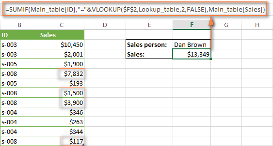
   

Download this VLOOKUP and SUMIF sample.

Formula-free way to do vlookup in Excel

Finally, let me introduce you the tool that can look up, match and merge your tables without any functions or formulas. The Merge Tables Wizard add-in was designed and develop as a time-saving and easy-to-use alternative to Excel's VLOOKUP and LOOKUP functions, and it can be very helpful both to beginners and advanced users.

Instead of figuring out formulas, you simply specify your main and lookup tables, define a common column or columns, and tell the wizard what data you want to fetch.

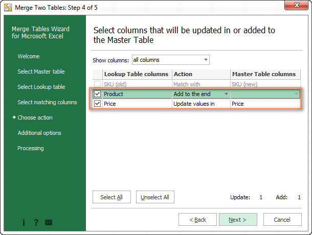
Then you allow the wizard a few seconds to look up, match and deliver you the results. If you think this add-in may prove helpful in your work, you are most welcome to download a trial version : )